4. Worked Example
This page provides a general overview of pysisyphus's capabilities for optimizing ground state reaction paths for the example of a tris-pericyclic reaction between a tropone derivative and dimethylfulvene.
You can find a short discussion of the reaction on Steven M. Bacharachs blog. Here we focus on how to obtain TS1. Instead of using DFT as in the original publication we'll employ the semi-emperical tight binding code xtb. It allows us to run all necessary calculations on common desktop hardware in little time (2 min, using 6 physical CPU cores).
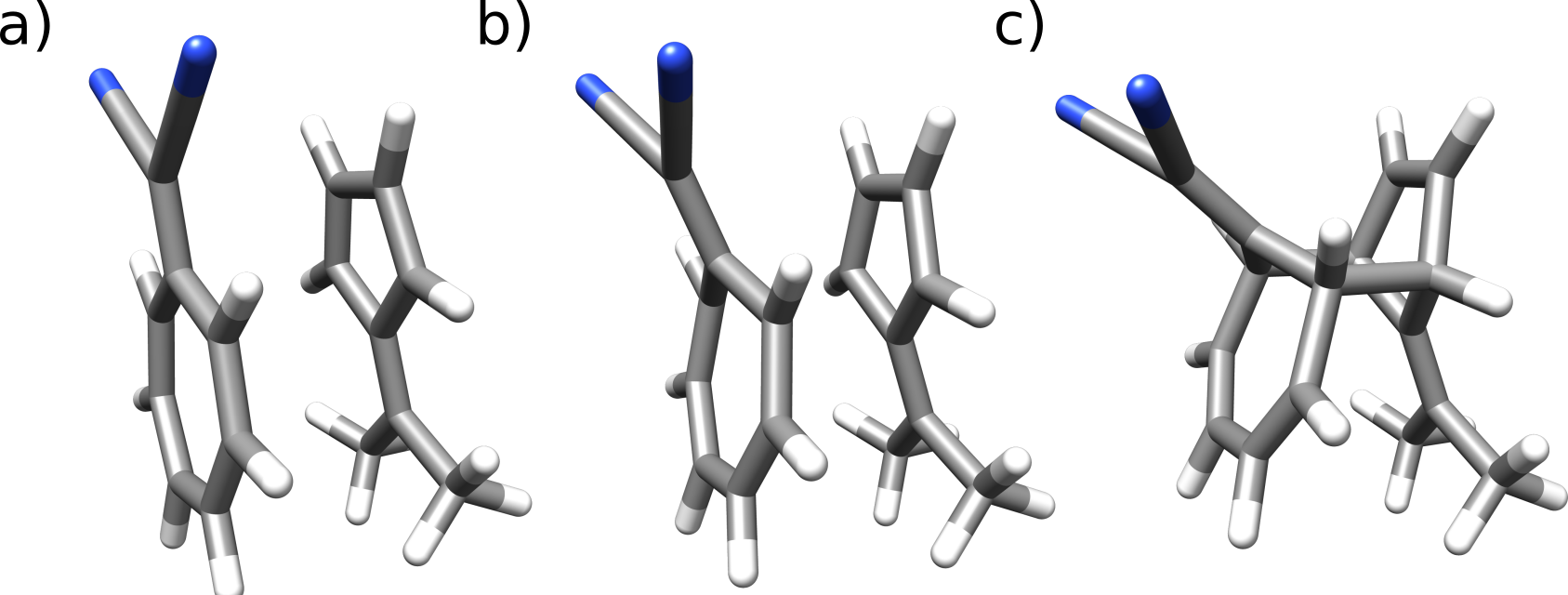
Fig. 4.1 Educts, TS and products of the tris-pericyclic reaction between a tropone derivative and dimethylfulvene.
At first, we have to create appropriate educt and product geometries using the molecular editor of our choice, e.g., avogadro or TmoleX. Given a reasonable educt geometry a suitable product geometry can be constructed by decreasing the distance between the two ring systems and optimizing the result, e.g., by xtb. Sometimes it may be easier to start with the product geometry, and obtain the educt from it. Consistent atom ordering in both geometries is mandatory! Usually it's a bad idea to construct both geometries independently, as it is easy to mess up the atom ordering.
Given educts (min_xtbopt.xyz) and product (prod_xtbopt.xyz) we can create the YAML input. Our goal is to obtain the barrier heights for the reaction shown in Fig. 4.1 by means of growing string (GS) calculation, transition state (TS) optimization, intrinsic reaction coordinate (IRC) calculation and subsequent optimization of the IRC endpoints. The full input is shown below. We'll go over it step by step.
geom:
 type: dlc
 fn: [min_xtbopt.xyz, prod_xtbopt.xyz]
preopt:
cos:
 type: gs
 max_nodes: 18
 climb: True
opt:
 type: string
 align: False
 max_cycles: 20
tsopt:
 type: rsirfo
 do_hess: True
 thresh: gau
 hessian_recalc: 3
irc:
 type: eulerpc
 rms_grad_thresh: 0.0005
endopt:
calc:
 type: xtb
 pal: 6
The desired coordinate system and the file names of the input geometries are given in the
geom block.
geom:
 type: dlc
 fn: [min_xtbopt.xyz, prod_xtbopt.xyz]
Here we chose delocalized internal coordiantes (DLC) for our GS, which is the
preferred way. Alternatively Cartesian coordinates could be used by
type: cart. If DLCs fail, Cartesian coordinates should be tried.
preopt:
The preopt block is given without any additional keywords, so sane defaults will
be used for preoptimizing educt and product geometries (Rational function
optimization (RFO) in redundant internal coordinates). Strictly, in our case preoptimization
is not necessary, as we already preoptimized the geometries using xtb. But in general
if is advised to span chain of states (COS) like GS or nudged elastic band (NEB) between
stationary points on the potential energy surface.
If the educts and products are NOT covalently bound it may be a good idea to restrict the
number of preoptimization cycles to a small number (max_cycles: 10), as these
optimizations are sometimes hard to converge. Please see Optimization of Minima
for a list of possible keywords in the preopt block.
cos:
 type: gs
 max_nodes: 18
 climb: True
The cos block configures COS calculations. Here we request a GS (gs)
with 18 nodes (images) between educt and product, resulting in a total string length
of 20 nodes. By default first and last node (educt and product) are kept fixed
throughout the optimization. We enable a climbing image (CI) to obtain a better TS guess.
Please see Chain Of States Methods for further information on COS methods.
opt:
 type: string
 align: False
 max_cycles: 20
COS/GS optimization is controlled via the opt block. For GS optimization one should always
use type: string. In internal coordinates we disable automated geometry alignment,
as it is not needed. We also restrict the number of optimization cycles to 20 (default 50).
The chosen optimizer will do steepest descent (SD) steps when the string grew in the previous
cycle, otherwise conjugate gradient (CG) steps are used. When the GS is fully grown/connected
the optimizer will use limited-memory Broyden-FletcherGoldfarb-Shanno (L-BFGS) to determine
more sophisticated steps.
tsopt:
 type: rsirfo
 do_hess: True
 thresh: gau
 hessian_recalc: 3
After GS convergence the highest energy image (HEI) is determined by cubic splining
and used as guess for a classical TS optimization using restricted step image RFO (RSIRFO).
do_hess: True requests a frequency calculation after the TS optimization.
The Hessian is recalculated every 3th step. When the Hessian for the chosen computational
method is reasonably cheap it is a good idea to recalculate it periodically.
Between recalculations it's updated using the Bofill-update. Convergence critera are
tightened from the default thresh: gau_loose to thresh: gau.
irc:
 type: eulerpc
 rms_grad_thresh: 0.0005
IRC integration is controlled in the irc block. By default the Euler-predictor-corrector
(EulerPC) integrator is used. Integration is terminated when the root-mean-square (RMS) of the
gradient is equal to or less than 0.0005 au. Possible inputs are given in
Intrinsic Reaction Coordinate (IRC).
endopt:
Similar to preopt the endopt will be executed with default arguments. It
is used to optimize the IRC endpoints to stationary points and enables printing of
additional information like RMS deviation of atomic positions (RMSD) between optimized
endpoints and initial geometries. The RMSD values help in deciding if the obtained TS
actually connects presumed educts and products.
calc:
 type: xtb
 pal: 6
The calc block configures the level of theory used in energy/gradient/Hessian
calculations. Here we chose xtb and requested 6 CPU cores. Additional inputs for
xtb can be found in the xtb module documentation
With everything set up we are ready to actually execute pysisyphus! Assuming the above YAML is saved to 01_pericyclic.yaml just run
pysis 01_pericyclic.yaml | tee pysis.log
By default pysisyphus prints to STDOUT so you have to capture STDOUT explicitely. We use
tee so everything is logged to a file and printed simulatenously.
A lot of files and output will be produced so we will go over everything slowly.
                           d8b                            888
                           Y8P                            888
                                                          888
88888b.  888  888 .d8888b  888 .d8888b  888  888 88888b.  88888b.  888  888 .d8888b
888 "88b 888  888 88K      888 88K      888  888 888 "88b 888 "88b 888  888 88K
888  888 888  888 "Y8888b. 888 "Y8888b. 888  888 888  888 888  888 888  888 "Y8888b.
888 d88P Y88b 888      X88 888      X88 Y88b 888 888 d88P 888  888 Y88b 888      X88
88888P"   "Y88888  88888P' 888  88888P'  "Y88888 88888P"  888  888  "Y88888  88888P'
888           888                            888 888
888      Y8b d88P                       Y8b d88P 888
888       "Y88P"                         "Y88P"  888

Version 0.5.0.post1+450.g2c1654d3 (Python 3.8.5, NumPy 1.19.2, SciPy 1.5.2)
Git commit 2c1654d35d69e7b48ac4e9b00d38afd58a8bedd4
Executed at Tue Oct  6 10:08:30 2020 on 'your fancy hostname'

If pysisyphus benefitted your research please cite:

    https://doi.org/10.1002/qua.26390

Good luck!
You will be greeted by a banner and some information about your current installation,
which hopefully aids in reproducing your results later on, if needed. Then your input
is repeated, including default values that you did not explicitely set. There you can
also see the default values chosen for preopt and endopt.
{'calc': {'pal': 6, 'type': 'xtb'},
 'cos': {'climb': True, 'fix_ends': True, 'max_nodes': 18, 'type': 'gs'},
 'endopt': {'dump': True,
            'fragments': False,
            'max_cycles': 100,
            'overachieve_factor': 3,
            'thresh': 'gau',
            'type': 'rfo'},
 'geom': {'fn': ['min_xtbopt.xyz', 'prod_xtbopt.xyz'], 'type': 'dlc'},
 'interpol': {'between': 0, 'type': None},
 'irc': {'rms_grad_thresh': 0.0005, 'type': 'eulerpc'},
 'opt': {'align': False, 'dump': True, 'max_cycles': 30, 'type': 'string'},
 'preopt': {'dump': True,
            'max_cycles': 100,
            'overachieve_factor': 3,
            'preopt': 'both',
            'strict': False,
            'thresh': 'gau_loose',
            'trust_max': 0.3,
            'type': 'rfo'},
 'tsopt': {'do_hess': True,
           'dump': True,
           'h5_group_name': 'tsopt',
           'hessian_recalc': 3,
           'overachieve_factor': 3,
           'thresh': 'gau',
           'type': 'rsirfo'}}
The whole run starts with preoptimizations of educt and product. Both optimizations converge quickly, as the geometries are already preoptimized.
                       #################################
                       # RUNNING FIRST PREOPTIMIZATION #
                       #################################
Spent 0.0 s preparing the first cycle.
cycle   max(force)    rms(force)     max(step)     rms(step)       s/cycle
    0     0.000080     0.000010     0.027005     0.003934          0.1
Converged!

Final summary:
            max(forces, internal): 0.000080 hartree/(bohr,rad)
            rms(forces, internal): 0.000010 hartree/(bohr,rad)
            max(forces,cartesian): 0.000063 hartree/bohr
            rms(forces,cartesian): 0.000015 hartree/bohr
            energy: -52.35197394 hartree
Wrote final, hopefully optimized, geometry to 'first_pre_final_geometry.xyz'

Preoptimization of first geometry converged!
Saved final preoptimized structure to 'first_preopt.xyz'.
RMSD with initial geometry: 0.000000 au

                        ################################
                        # RUNNING LAST PREOPTIMIZATION #
                        ################################
Spent 0.0 s preparing the first cycle.
cycle   max(force)    rms(force)     max(step)     rms(step)       s/cycle
    0     0.000188     0.000025     0.002310     0.000592          0.1
Converged!

Final summary:
            max(forces, internal): 0.000188 hartree/(bohr,rad)
            rms(forces, internal): 0.000025 hartree/(bohr,rad)
            max(forces,cartesian): 0.000182 hartree/bohr
            rms(forces,cartesian): 0.000032 hartree/bohr
            energy: -52.39960456 hartree
Wrote final, hopefully optimized, geometry to 'last_pre_final_geometry.xyz'

Preoptimization of last geometry converged!
Saved final preoptimized structure to 'last_preopt.xyz'.
RMSD with initial geometry: 0.000000 au
After an optimization remaining RMS and max of the forces are reported for internal and
Cartesian coordinates. If the internal force is zero, but a substantial Cartesian
force remains someting went wrong, e.g., the generated coordinate system is lacking
important coordinates. In such cases the generated coordinates can be examined manually
pysistrj [geom file] --internals to determine important missing coordinates.
Preoptimizations are followed by the GS optimization.
                           #########################
                           # RUNNING GROWINGSTRING #
                           #########################
Spent 0.0 s preparing the first cycle.
cycle   max(force)    rms(force)     max(step)     rms(step)       s/cycle
    0     0.006403     0.001545     0.006403     0.001545          0.2
    String=2+2 HEI=02/04 (E_max-E_0)=1.4 kJ/mol
    1     0.009367     0.001734     0.009367     0.001734          0.3
    String=3+3 HEI=03/06 (E_max-E_0)=4.1 kJ/mol
    2     0.010394     0.001807     0.010394     0.001807          0.6
    String=4+4 HEI=04/08 (E_max-E_0)=8.0 kJ/mol
    3     0.011152     0.001790     0.011152     0.001790          1.1
    String=5+5 HEI=05/10 (E_max-E_0)=12.5 kJ/mol
    4     0.010687     0.001722     0.010687     0.001722          1.0
    String=6+6 HEI=06/12 (E_max-E_0)=17.6 kJ/mol
    5     0.008751     0.001620     0.008751     0.001620          1.1
    String=7+7 HEI=07/14 (E_max-E_0)=22.8 kJ/mol
    6     0.008007     0.001517     0.008007     0.001517          1.3
    String=8+8 HEI=08/16 (E_max-E_0)=27.6 kJ/mol
    7     0.006895     0.001423     0.006895     0.001423          1.4
    String=9+9 HEI=09/18 (E_max-E_0)=31.3 kJ/mol
Starting to climb in next iteration.
    8     0.006253     0.001313     0.006253     0.001314          1.6
    String=Full HEI=10/20 (E_max-E_0)=32.8 kJ/mol
    9     0.006134     0.001169     0.059438     0.011487          1.7
    String=Full HEI=10/20 (E_max-E_0)=32.0 kJ/mol
   10     0.009555     0.001504     0.022529     0.003827          1.6
    String=Full HEI=10/20 (E_max-E_0)=31.6 kJ/mol
   11     0.009792     0.001583     0.100000     0.011614          1.7
    String=Full HEI=10/20 (E_max-E_0)=31.6 kJ/mol
   12     0.008636     0.001534     0.100000     0.011518          1.7
    String=Full HEI=10/20 (E_max-E_0)=30.7 kJ/mol
   13     0.008708     0.001448     0.100000     0.011463          1.6
    String=Full HEI=10/20 (E_max-E_0)=30.0 kJ/mol
   14     0.008217     0.001363     0.100000     0.005660          1.7
    String=Full HEI=10/20 (E_max-E_0)=29.4 kJ/mol
   15     0.007743     0.001335     0.100000     0.005297          1.7
    String=Full HEI=10/20 (E_max-E_0)=29.1 kJ/mol
   16     0.007243     0.001307     0.100000     0.005143          1.6
    String=Full HEI=10/20 (E_max-E_0)=28.8 kJ/mol
   17     0.006897     0.001285     0.100000     0.004938          1.6
    String=Full HEI=10/20 (E_max-E_0)=28.6 kJ/mol
   18     0.006772     0.001277     0.100000     0.004992          1.6
    String=Full HEI=10/20 (E_max-E_0)=28.5 kJ/mol
   19     0.006714     0.001273     0.100000     0.005006          1.6
    String=Full HEI=10/20 (E_max-E_0)=28.5 kJ/mol
Found sign 'converged'. Ending run.
Operator indicated convergence!
Wrote final, hopefully optimized, geometry to 'final_geometries.trj'
Splined HEI is at 8.07/19.00, between image 8 and 9 (0-based indexing).
Wrote splined HEI to 'splined_hei.xyz'
The string grows quickly and is fully grown in cycle 8. String size and barrier height between the first and HEI are reported in every cycle. From cycle 8 on, a CI is employed. The final HEI index is printed at the end. As we interpolate the HEI, the index may be a fractional number. The COS optimization is followed by a TS optimization.
                      ####################################
                      # RUNNING TS-OPTIMIZATION FROM COS #
                      ####################################
Creating mixed HEI tangent, using tangents at images (8, 9).
Overlap of splined HEI tangent with these tangents:
    08: 0.982763
    09: 0.149474
Index of splined highest energy image (HEI) is 8.07.

Wrote animated HEI tangent to cart_hei_tangent.trj

Splined HEI (TS guess)
[xyz file printed here; removed for clarity]

Splined Cartesian HEI tangent
[xyz file printed here; removed for clarity]

Wrote splined HEI coordinates to 'splined_hei.xyz'
Calculating Hessian at splined TS guess.
Negative eigenvalues at splined HEI:
[-0.005069 -0.000317]
Overlaps between HEI tangent and imaginary modes:
    00: 0.856746
    01: 0.009826
Imaginary mode 0 has highest overlap with splined HEI tangent.
Spent 0.3 s preparing the first cycle.
cycle   max(force)    rms(force)     max(step)     rms(step)       s/cycle
    0     0.009004     0.001343     0.056873     0.017930          0.2
    1     0.000754     0.000227     0.158373     0.035866          0.2
    2     0.001142     0.000156     0.316150     0.051562          3.6
    3     0.000483     0.000082     0.339089     0.052646          0.2
    4     0.000370     0.000067     0.321142     0.049527          0.2
    5     0.000362     0.000050     0.243173     0.040395          3.6
    6     0.000152     0.000023     0.174987     0.032910          0.2
    7     0.000503     0.000063     0.092082     0.019454          0.2
    8     0.000199     0.000031     0.121285     0.024502          3.5
    9     0.000136     0.000019     0.061690     0.012096          0.2
Converged!

Final summary:
            max(forces, internal): 0.000136 hartree/(bohr,rad)
            rms(forces, internal): 0.000019 hartree/(bohr,rad)
            max(forces,cartesian): 0.000164 hartree/bohr
            rms(forces,cartesian): 0.000043 hartree/bohr
            energy: -52.34823514 hartree
Wrote final, hopefully optimized, geometry to 'ts_final_geometry.xyz'
Optimized TS coords:
[xyz file printed here; removed for clarity]

Wrote TS geometry to 'ts_opt.xyz'

                         -----------------------------
                         | HESSIAN AT FINAL GEOMETRY |
                         -----------------------------

... mass-weighing cartesian hessian
... doing Eckart-projection

First 10 eigenvalues [-2.4303e-03 -3.9622e-17 -8.1858e-18 -7.8671e-19  2.1865e-18  5.1589e-18
  2.6247e-17  1.3733e-05  7.3736e-05  1.2735e-04]
Imaginary frequencies: [-253.24] cm⁻¹

Wrote final (not mass-weighted) hessian to 'calculated_final_cart_hessian'.
Wrote HD5 Hessian to 'final_hessian.h5'.
Wrote imaginary mode with ṽ=-253.24 cm⁻¹ to 'imaginary_mode_000.trj'

Barrier between TS and first COS image: 9.8 kJ mol⁻¹
Barrier between TS and last COS image: 134.9 kJ mol⁻¹
The initial HEI TS guess features only two sizable imaginary frequencies, confirming that
it is a suitable TS guess. Root 0 has the highest overlap (85%) with the HEI tangent and is
chosen for maximization in the TS optimization, whereas the energy will be minimized along
the remaining modes. The optimization converged quickly in 10 cycles. A final Hessian is
computed at the optimized TS as we used do_hess: True. Only one imaginary frequency
remains, which is the desired result for a first-order saddle point. All sizable imaginary
modes are written to .trj files and can be viewed by tools like jmol.
Barrier heights between the TS and first and last COS image (no thermochemistry is included!) are reported. In this case the energy difference between the first COS image and the TS is very small, indicating an early TS, similar to the educts. This is also be confirmed by examining Fig. 4.1.
                                ###############
                                # RUNNING IRC #
                                ###############
Calculating energy and gradient at the TS
IRC length in mw. coords, max(|grad|) and rms(grad) in unweighted coordinates.
Norm of initial displacement step: 0.1974

                               #################
                               # IRC - FORWARD #
                               #################

        Step   IRC length      dE / au  max(|grad|)    rms(grad)
        --------------------------------------------------------
           0     0.298147    -0.000333     0.001413     0.000394
        Integrator indicated convergence!

                               ##################
                               # IRC - BACKWARD #
                               ##################

        Step   IRC length      dE / au  max(|grad|)    rms(grad)
        --------------------------------------------------------
           0     0.332823    -0.000938     0.004607     0.001154
           1     0.662398    -0.001367     0.006116     0.001608
           2     0.991868    -0.001878     0.008670     0.002208
           3     1.320005    -0.002558     0.012581     0.002968
           4     1.644982    -0.003249     0.015719     0.003595
           5     1.966058    -0.003700     0.017023     0.003976
           6     2.285006    -0.003972     0.016598     0.004230
           7     2.596325    -0.004126     0.019112     0.004415
           8     2.898296    -0.004206     0.021118     0.004439
           9     3.186446    -0.004052     0.021182     0.004240
          10     3.462246    -0.003697     0.019162     0.003793
          11     3.723777    -0.003087     0.015042     0.003078
          12     3.966373    -0.002263     0.009324     0.002161
          13     4.173308    -0.001387     0.003822     0.001310
          14     4.321559    -0.000781     0.002226     0.000838
          15     4.420391    -0.000523     0.001616     0.000642
          16     4.498118    -0.000418     0.001299     0.000548
          17     4.571712    -0.000353     0.001967     0.000569
          18     4.647481    -0.000298     0.004516     0.000754
          19     4.722445    -0.000308     0.003469     0.000670
          20     4.808189    -0.000290     0.003426     0.000682
          21     4.881593    -0.000209     0.004155     0.000683
        Integrator indicated convergence!
The imaginary mode is used to displace the TS towards educts and product.
As the TS is very similar to the educt, forward IRC integration already terminates after
one cycle. Maybe, further integration steps could be forced by tightening the threshold
in the irc: block. Backward integration terminates after 22 cycles. At first,
the gradient increases and after the inflection point is passed, falls off again as
a stationary point is approached. In the end both IRC endpoints are fully optimized to
stationary points.
                      ####################################
                      # RUNNING FORWARD_END OPTIMIZATION #
                      ####################################
Spent 0.0 s preparing the first cycle.
cycle   max(force)    rms(force)     max(step)     rms(step)       s/cycle
    0     0.000491     0.000126     0.099615     0.030780          0.1
    1     0.001769     0.000333     0.121277     0.033041          0.2
    2     0.002986     0.000525     0.228218     0.054622          0.2
    3     0.002455     0.000475     0.396872     0.096049          0.2
    4     0.003106     0.000502     0.061397     0.012734          0.2
    5     0.000676     0.000187     0.040565     0.007988          0.2
    6     0.000498     0.000144     0.048609     0.012294          0.2
    7     0.000908     0.000142     0.055895     0.016806          0.2
    8     0.000715     0.000102     0.037441     0.011352          0.2
    9     0.000226     0.000047     0.034467     0.006157          0.2
   10     0.000119     0.000032     0.034646     0.006157          0.1
Converged!

Final summary:
            max(forces, internal): 0.000119 hartree/(bohr,rad)
            rms(forces, internal): 0.000032 hartree/(bohr,rad)
            max(forces,cartesian): 0.000241 hartree/bohr
            rms(forces,cartesian): 0.000073 hartree/bohr
            energy: -52.35194671 hartree
Wrote final, hopefully optimized, geometry to 'forward_end_final_geometry.xyz'

Moved 'forward_end_final_geometry.xyz' to 'forward_end_opt.xyz'.

                     #####################################
                     # RUNNING BACKWARD_END OPTIMIZATION #
                     #####################################
Spent 0.0 s preparing the first cycle.
cycle   max(force)    rms(force)     max(step)     rms(step)       s/cycle
    0     0.004485     0.001075     0.168005     0.031009          0.1
    1     0.003805     0.000731     0.158516     0.028598          0.2
    2     0.003345     0.000610     0.047413     0.008626          0.2
    3     0.002849     0.000531     0.093820     0.017252          0.2
    4     0.001571     0.000332     0.154150     0.028740          0.2
    5     0.000752     0.000148     0.034367     0.007031          0.2
    6     0.000630     0.000107     0.017362     0.004137          0.2
    7     0.000218     0.000047     0.019096     0.003624          0.1
    8     0.000165     0.000041     0.027156     0.004814          0.2
    9     0.000400     0.000065     0.044195     0.007618          0.2
   10     0.000460     0.000076     0.039724     0.006652          0.1
   11     0.000265     0.000059     0.021454     0.003444          0.2
   12     0.000194     0.000034     0.009649     0.001594          0.1
   13     0.000146     0.000025     0.009711     0.001835          0.1
Converged!

Final summary:
            max(forces, internal): 0.000146 hartree/(bohr,rad)
            rms(forces, internal): 0.000025 hartree/(bohr,rad)
            max(forces,cartesian): 0.000183 hartree/bohr
            rms(forces,cartesian): 0.000047 hartree/bohr
            energy: -52.39959356 hartree
Wrote final, hopefully optimized, geometry to 'backward_end_final_geometry.xyz'

Moved 'backward_end_final_geometry.xyz' to 'backward_end_opt.xyz'.
Both optimizations converge quickly without any problems. Finally, optimized endpoint geometries are compared to the intial geometries and final barrier heights are reported. Thermochemistry is not (yet) included. Even though both endpoints are reported as dissimilar to the initial geomtries they are still very similar, confirming, that the obtained TS indeed connects presumed educts and product.
                       #################################
                       # RMSDS AFTER END OPTIMIZATIONS #
                       #################################
start geom  0 (first_preopt.xyz/min_xtbopt.xyz)
    end geom  0 ( forward_end_opt.xyz): RMSD=0.133727 au
    end geom  1 (backward_end_opt.xyz): RMSD=1.126059 au
    Optimized end geometries are dissimilar to 'first_preopt.xyz/min_xtbopt.xyz'!
start geom  1 (last_preopt.xyz/prod_xtbopt.xyz)
    end geom  0 ( forward_end_opt.xyz): RMSD=1.144102 au
    end geom  1 (backward_end_opt.xyz): RMSD=0.093044 au
    Optimized end geometries are dissimilar to 'last_preopt.xyz/prod_xtbopt.xyz'!

                  ###########################################
                  # BARRIER HEIGHTS AFTER END OPTIMIZATIONS #
                  ###########################################
Thermochemical corrections are NOT included!

Minimum energy of 0.0 kJ mol⁻¹ at 'backward_end_opt.xyz'.

     forward_end_opt.xyz:   125.10 kJ mol⁻¹
                      TS:   134.84 kJ mol⁻¹
    backward_end_opt.xyz:     0.00 kJ mol⁻¹

Wrote optimized end-geometries and TS to 'end_geoms_and_ts.trj'
Visualization/plotting of running optimizations and IRC integrations is also possible. Please see Plotting for further information.
All inputs can be found in the examples/complex/08_trispericyclic directry on github.