15. Diabatiziation
Pysisyphus implements property-based diabatizion, as outlined by Subotnik [1] [2] and Truhlar et al. [3]
By determining a suitable rotation matrix \(\mathbf{U}\), adiabatic states can be mixed into diabatic states. In the context of property based diabatization, \(\mathbf{U}\) is determined to maximize a cost funtion \(f(\mathbf{U})\) that depends on a selected molecular property or a set thereof.
Given the repsective property tensors in the basis of the adiabatic states, diabatization can be carried out using dipole moments (Boys-diabatization), the trace of the of the primitive quadrupole tensor and the electrostatic potential (DQ \(\Phi\)-diabatization), or using the Coulomb-tensor (Edmiston-Ruedenberg (ER) diabatization). An extension to ER-diabatization called \(\varepsilon\)-ER that takes temperature and a solvent parameter (Pekar factor \(C\)) into account was also proposed. [4] By setting the temperature to a very high value, plain ER-diabatization is recovered when using \(\varepsilon\)-ER.
Currently, pysisyphus provides two diabatization-interfaces: a legacy YAML-interface where all required properties must be provided by the user and a newer one, where the properties are calculated automatically.
The legacy YAML-interface allows DQ \(\Phi\)-diabatization, whereas the newer interface allows (\(\varepsilon\))-ER and plain Boys-diabatization. The newer interface requires only a single TDA/TD-DFT calculation yielding a wavefunction, transition density matrices and adiabatic state energies. Currently, the newer interface is restricted to TDA/TDDFT-like calculations carried out by ORCA 5.0.4. As the calculation of the Coulomb-tensor is computationally expensive it is not implemented in Python, but in Fortran via the pysisyphus-addons project.
For the ER-diabatization to work, the pysisyphus-addons must be installed. The easiest way to achive this, is to use Nix (see Installation via Nix).
15.1. General Idea
15.1.1. Rotation Matrix
Diabatic states \(\{\Xi_A\}\) can be obtained via unitary transformation of adiabatic states \(\{\Psi_I\}\).
which in matrix notation is equivalent to
with rotation matrix \(\mathbf{U}\), as well as adiabatic and diabatic state vectors \(\mathbf{\Psi}\) and \(\mathbf{\Xi}\). Given two adiabatic states \(\Psi_1\) and \(\Psi_2\) \(\mathbf{U}\) is defined as
The related diabatic states \(\Xi_A\) and \(\Xi_B\) are
Similarly, diabatic expectation values are calculated as linear combination of adiabatic expectation values:
or in matrix notation
By maximizing a cost function that depends on diabatic properties \(\mathbf{O}_\mathrm{dia}\), a rotation matrix \(\mathbf{U}\) suitable for diabatization can be determined.
With a known rotation matrix \(\mathbf{U}\), the diagonal adiabatic electronic energy matrix \(\mathbf{V}\) can be transformed to its diabatic equivalent \(\mathbf{D}\), e.g, to determine diabatic couplings \(|D_{12}|\).
15.1.2. Cost function
Depending on the employed properties, different cost functions \(f(\mathbf{U})\) are used. Subotnik [2] proposed to maximize the magnitude of the diabatic dipole moments:
This is the same cost function as in classical Boys localization of molecular orbitals. By also considering the trace of the primitive quadrupole tensor, \(f_D(\mathbf{U})\) is extended to \(f_{DQ}(\mathbf{U})\):
The contribution of the quadrupole moments to \(f(\mathbf{U})\) is controlled by the scaling factor \(\alpha_j\). Here, subscript \(j\) refers to the j-th expansion center. Currently, only one expansion center (\(N_Q = 1\)) can be used in pysisyphus. By default \(\alpha_j\) is set to \(10 ~ a_0^{-2}\).
In some cases, considering only the dipole moments is not enough to discriminate different adiabatic states and quadrupole moments have to be taken into account. Several examples are outlined by Truhlar et al. [3]
Slight improvements may be possible by incorporating the electronic component of the electrostatic potential (ESP) \(\Phi\).
Here again, \(N_\Phi\) denotes the number of expansion centers where the ESP is calculated. Similar to the quadrupole moments, only one expansion center is currently supported in pysisyphus. \(\beta_k\) is a scaling factor that controls the contribution of the electrostatic potential to the overall cost function \(f_{DQ\Phi}(\mathbf{U})\).
In the case of ER-diabatization the cost function is given by
with diabatic state index \(A\), adiabatic state labels \(I, J, K, L\) and molecular orbitals (MOs) labels \(r, s, p, q\), as well as density matrices \(P^{IJ}_{rs}\) (see Densities).
As there are often just a few adiabatic states (\(\ll 10\)) but many MOs, the computational bottleneck is the calculation of the Coulomb-tensor. In the current implementation, the Coulomb-tensor is calculated using density fitting, as outlined in the Appendix of [1]. By default, density fitting integrals are available up to \(\left( GG|H \right)\), that is up to \(G\) functions in the principal basis and up to \(H\) functions in the auxiliary basis. The auxiliary basis is hardcoded to def2/J [9] and cannot be modified by the user. Similarly, Coulomb-integrals for Schwarz-Screening are available up to \(\left(GG|GG\right)\)
15.1.3. Cost Function Optimization
There are different approaches on how to optimize the cost-function.
Probably the oldest approach to maximize the cost function \(f\) is achieved via repeated 2 x 2 rotations (Jacobi sweeps) of diabatic state pairs. The formulas to calculate the required rotation angle are given by Kleier [5] and Pulay et al., [6] as well as Edmiston and Ruedenberg. [7] The maximization is started with a unit-matrix guess for \(\mathbf{U}\) and usually converges quite rapidly.
A different approach is outlined by Folkestad. [8] The orthogonal rotation matrix \(\mathbf{U}\) can be parametrized as the matrix exponential of a real-valued antisymmetric matrix \(\boldsymbol{\kappa}\).
When the gradient of the cost function \(f(\mathbf{U}(\boldsymbol{\kappa}))\) w.r.t. to \(\boldsymbol{\kappa}\) is available, all standard optimization techniques can be applied. For the \(\varepsilon\)-ER diabatization, pysisyphus utilizes jax to determine the gradient and the Hessian of the cost function \(f_\mathrm{ER}(\mathbf{U(\boldsymbol{\kappa})})\).
The cost function is then optimized using the Newton-CG method from scipy. By also taking the Hessian into account we can ensure that we actually converge to a true maximum, with only negative Hessian eigenvalues.
15.1.4. Densities
The relevant molecular properties in the basis of the adiabatic states are calculated by contracting the adiabatic densities with the respective integrals, e.g. dipole moment integrals, or Coulomb-integrals. A density matrix element in the molecular orbital basis between two states \(I\) and \(J\) is given as
with \(c^\dagger_r\) and \(c_s\) being creation and annihilation operators for orbitals \(r\) and s. \(t^{Jr}_a\) is an element of the (unrelaxed) transition density tensor for a transition between occupied MO \(a\) and virtual MO \(r\) in the excitation from the GS to state \(J\). [1] For TDA/TD-DFT-like states, \(t^{Jr}_a\) corresponds to \((X+Y)^{Jr}_a\) with \(\boldsymbol{Y}\) being a zero matrix in the case of TDA/CIS. In the case of \(\varepsilon\)-ER the \(\delta_{rs} \delta_{JK}\) part is neglected. [4]
In the current implementation, all densities are expressed in the atomic orbital (AO) basis.
15.2. Legacy YAML Interface
All possible input options are outlined below. The numbers are just dummy values. See Legacy YAML Interface - Example for an actual example.
# Adiabatic energies, of the states to diabatize.
#
# List of floats.
#   [V0, V1, ...]
# May be absolute or relative energies.
adiabatic_energies: [0.0, 0.6541, 0.7351]
# Dipole moments.
#
# List of lists of length 5, each containing 2 integers followed by 3 floats.
#   [state0, state1, dpm_x, dpm_y, dpm_z]
# The integers are adiabatic state indices, the 3 floats are the X, Y and Z
# components of a dipole moment vector.
# If both integers are the same, the 3 floats correspond to the permanent dipole moment
# of a state. Otherwise, they correspond to a transition dipole moment
# between two states.
dipoles: [
 [0, 0, -1.0, -2.0, -3.0],
 [1, 1, -2.0, -1.0, -3.0],
 [0, 1, -2.0, -1.0, -3.0],
]

#
# Optional input below
#

# Adiabatic state labels.
#
# List of strings.
#   [label1, label2, ...]
# Must be of same length as adiabatic energies.
adiabiatc_labels: [GS, LE, CT]
# Energy unit.
#
# Literal["eV", "Eh"]
unit: eV
# Trace of primitive quadrupole moment tensor.
#
# List of lists of length 3, each containing 2 integers followed by 1 float.
#   [state0, state1, tr_qpm] = [state0, state1, (qpm_xx + qpm_yy + qpm_zz)
# The same comments as for the dipole moments apply.
quadrupoles: [
 [0, 0, 1.0],
 [1, 1, -14.0],
 [0, 1, 33.0],
]
# Quadrupole moment scaling factor alpha in 1/a₀².
#
# Float
alpha: 10.0
# Electronic component of electrostatic potential in au
epots: [
 [0, 0.48],
 [1, 0.12],
]
# Electrostatic potential scaling factor beta in a₀.
#
# Float
beta: 1.0
15.3. Legacy YAML Interface - Example
Diabatization of 3 adiabatic states using dipole moments requires the 3 adiabatic permanent dipole moments (0,0; 1,1; 2,2), as well as the respective transition dipole moments (0,1; 0,2; 1,2).
# Guanine-Indole cation, wB97X-D/6-31G*, TDA, 3 states.
# Values are taken from the Table S2 in the SI of
# https://doi.org/10.1063/5.0035593
adiabatic_energies: [0.0, 0.717, 0.905]
adiabatic_labels: [GS, LE, CT]
dipoles:
  - [0, 0, -1.253, 0.270, -1.876]
  - [1, 1, -1.691, -0.653, -2.083]
  - [2, 2, 0.948, 0.733, -1.327]
  - [0, 1, -1.224, -0.279, -0.325]
  - [0, 2, 2.227, 0.866, 0.735]
  - [1, 2, -1.574, -1.029, -0.517]
Executing pysisdia guanine_indole_dia.yaml produces the following output:
                          ###################
                          # D-DIABATIZATION #
                          ###################

Dipole moments
--------------
[[[-1.253 -1.224  2.227]
  [-1.224 -1.691 -1.574]
  [ 2.227 -1.574  0.948]]

 [[ 0.27  -0.279  0.866]
  [-0.279 -0.653 -1.029]
  [ 0.866 -1.029  0.733]]

 [[-1.876 -0.325  0.735]
  [-0.325 -2.083 -0.517]
  [ 0.735 -0.517 -1.327]]]

Starting Jacobi sweeps.
000: P= 31.80729200 dP=         nan
001: P=169.63193103 dP=137.82463903
002: P=172.49529007 dP=  2.86335904
003: P=172.49529008 dP=  0.00000000
Jacobi sweeps converged after 3 macro cycles.

########################
# DIABATIZATION REPORT #
########################

Kind: dq

All energies are given in eV.

Every column of the rotation matrix U describes the composition of
a diabatic state in terms of (possibly various) adiabatic states.

Adiabatic energy matrix V
-------------------------
[[  0.000000   0.000000   0.000000]
 [  0.000000   0.717000   0.000000]
 [  0.000000   0.000000   0.905000]]

Rotation matrix U
-----------------
[[  0.8492   0.5023   0.1629]
 [  0.3860  -0.3800  -0.8406]
 [ -0.3603   0.7767  -0.5166]]
det(U)=1.0000

Diabatic energy matrix D = UᵀVU
-------------------------------
[[  0.224350  -0.358467  -0.064184]
 [ -0.358467   0.649500  -0.134102]
 [ -0.064184  -0.134102   0.748149]]

Diabatic states Ξᵢ sorted by energy
-----------------------------------
0: Ξ₀, 0.2244 eV
1: Ξ₁, 0.6495 eV
2: Ξ₂, 0.7481 eV

Composition of diabatic states Ξᵢ
---------------------------------
Ξ₀ = + 0.8492·Φ₀(GS) + 0.3860·Φ₁(LE) - 0.3603·Φ₂(CT)
Ξ₁ = + 0.5023·Φ₀(GS) - 0.3800·Φ₁(LE) + 0.7767·Φ₂(CT)
Ξ₂ = + 0.1629·Φ₀(GS) - 0.8406·Φ₁(LE) - 0.5166·Φ₂(CT)

Weights U²
----------
[[  0.7211   0.2523   0.0265]
 [  0.1490   0.1444   0.7066]
 [  0.1298   0.6033   0.2669]]

Unique absolute diabatic couplings
----------------------------------
|D₀₁| = 0.35847 eV, ( 2891.23 cm⁻¹)
|D₀₂| = 0.06418 eV, (  517.68 cm⁻¹)
|D₁₂| = 0.13410 eV, ( 1081.61 cm⁻¹)
15.4. New Interface
The new diabatiazation driver is available via python -m pysisyphus.diabatization.driver.
It implements \((\varepsilon)\)-ER and plain Boys-diabatization, with automatic calculation of the required property tensors. For visualization purposes it also implements the calculation of various adiabatic and diabatic cubes.
Before running any ER-diabatization it is important to increase any stack size limits with
ulimit -s unlimited
otherwise the calculation of the Coulomb-tensor is likely to crash.
While the pysisyphus-addons package is required to obtain the Coulomb-tensor, the integrals for Boys-diabatization are calculated using numba-accelerated functions. For both methods the integral calculation is parallelized. The number of threads for the calculation of the Coulomb-tensor can be controlled by setting the environment variable OMP_NUM_THREADS to a reasonable value.
Even though the calculation of dipole moment integrals is computationally much less challenging, there may still be some performance gains by varying the threading layer that numba uses. Personally, I found the omp threading layer to be the fastest. See the numba documentation for more information.
Available options for pysisyphus.diabatization.driver are given below:
$ python -m pysisyphus.diabatization.driver -h

usage: driver.py [-h] --states STATES [STATES ...] [--triplets] [--ovlp] [--dia DIA [DIA ...]] [-T TEMPERATURE] [-C PEKAR] [--cube CUBE [CUBE ...]] [--grid-points GRID_POINTS] [--out-dir OUT_DIR] orca_outs [orca_outs ...]

positional arguments:
  orca_outs

--states STATES [STATES ...]
                      Adiabatic state indices to use in the diabatization process. The GS corresponds to 0.
--triplets            Flag to indicate if the calculation contains singlet-triplet excitations.
--ovlp                Determine states from tden-overlaps between steps.
--dia DIA [DIA ...]   Available diabatization algorithms: EDMISTON_RUEDENBERG, EDMISTON_RUEDENBERG_ETA, BOYS, HALF.
-T TEMPERATURE, --temperature TEMPERATURE
                      Temperature in K. Only required for EDMISTON_RUEDENBERG_ETA.
-C PEKAR, --pekar PEKAR
                      Pekar factor. Only required for EDMISTON_RUEDENBERG_ETA.
--cube CUBE [CUBE ...]
                      Available cubes (DA: detachment/attachment, SD: spin density): ADIA_DA, DIA_DA, ADIA_SD, DIA_SD, SD.
--grid-points GRID_POINTS
                      Number of grid points per cube axis.
--out-dir OUT_DIR     Write the generated files to this directory. Defaults to the cwd ('.').
Diabatization using multiple methods and/or calculation of different kinds of cubes can be carried out in one run by specifying multiple keys. The command --dia BOYS EDMISTON_RUEDENBERG requests two diabatizations using different methods and the command --cube ADIA_DA DIA_DA requests the calculation of adiabatic and diabatic detachment-attachment densities. Creation of detachment-attachment densities is skipped for the adiabatic ground state.
15.5. New Interface - Example 1
ER-diabatization is demonstrated for trans-OMP3, as discussed in [1]. The geometry used here belongs to the \(C_{2h}\) point group and was optimized at the HF/6-31G* level of theory.
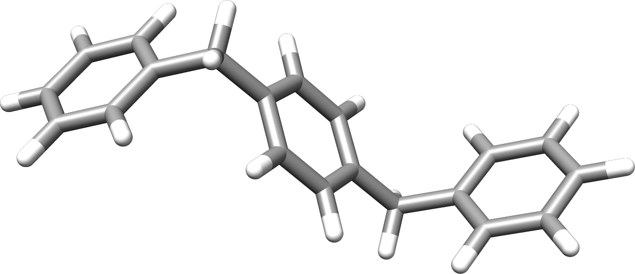
Fig. 15.1 OMP3 input structure optimized at the HF/6-31G* level of theory.
Looking at the detachment-attachment densities of the first 6 singlet excited adiabatic states calculated at the CIS/6-31G* level of theory, we find them highly mixed and spread out over multiple phenyl fragments.
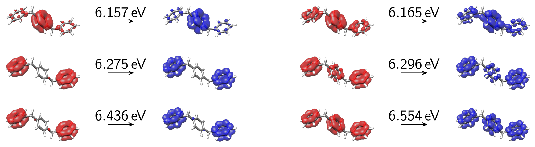
Fig. 15.2 Adiabatic detachment-attachment densities of the first 6 singlet excited states of OMP3 as obtained at the CIS/6-31G* level of theory.
ER-diabatization with the following command
#!/bin/bash
ulimit -s unlimited
OMP_NUM_THREADS=6 python -m pysisyphus.diabatization.driver 00_omp3_trans_c2h.log \
  --states 1 2 3 4 5 6 \
  --dia EDMISTON_RUEDENBERG \
  --cube ADIA_DA DIA_DA | tee tddia.log
produces the following diabatic detachment-attachment densities.
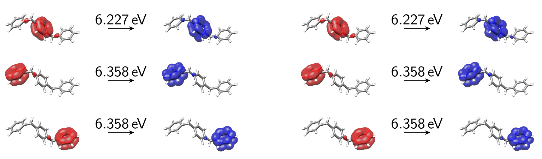
Fig. 15.3 Diabatic detachment-attachment densities of the first 6 singlet excited states of OMP3 as obtained at the CIS/6-31G* level of theory after ER-diabatization.
While pysisyphus can't create the detachment-attachment figures automatically it can visualize the diabatic couplings between the diabatic states using the graph library networkx. With one node per diabatic state and one edge per diabatic coupling a graph can be constructed. Due to the spatial dependence of the coupling strength between different diabatic states (high separation, small coupling), a plot of such a graph can offer a quick impression of the coupling situation for a given system.
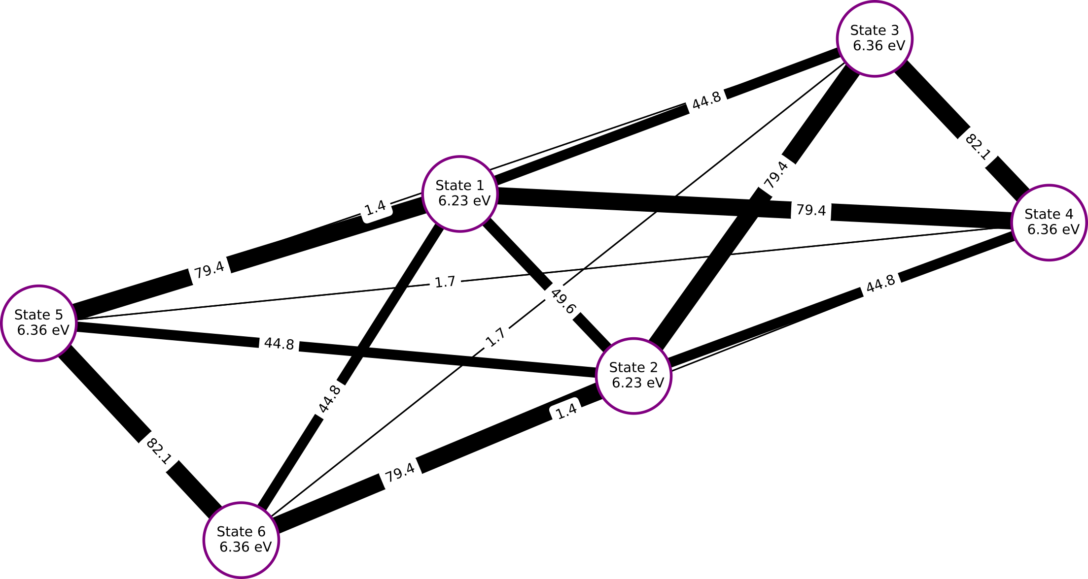
Fig. 15.4 Diabatic couplings for OMP3, as obtained from ER-diabatization. All couplings are given in meV. Please note that the positions of the 79.4 meV and 44.8 meV coupling edges are interchanged between the left and the right half of the plot. This is an artifact of the automatic generation of the plots.
The plot highlights the fact, that the coupling between adjacent phenyl fragments is much stronger than the coupling between the outer phenyl fragments. All results obtained with pysisyphus are fully in line with the reference results from [1].
15.6. New Interface - Example 2
An intersting example for property-based diabatization that involves the ground state from the HAB11 hole-transfer benchmark set of Kubas is shown below. [10] This example highlights the versatility of the current implementation, as it allows seamless inclusion of the ground state.
The geometry comprises a thiophene dimer, with the two thiophenes being separated by 5.0 Å. The geometry was taken from the supporting information of. [10] The calculation was carried out at the \(\omega`B97X-D/cc-pvtz/RIJCOSX level of theory using charge :math:`+1\) and doublet multiplicity. The first three excited states were calculated using TD-DFT. A stability analysis was required to converge to the actual ground state. The ground state \(D_0\) and the first excited doublet state \(D_1\) were considered in the ER-diabatization.
Executing
#!/bin/bash
ulimit -s unlimited
OMP_NUM_THREADS=6 python -m pysisyphus.diabatization.driver 01_thiophene_50_td_ro.log \
  --states 0 1 \
  --dia EDMISTON_RUEDENBERG \
  --cube ADIA_SD DIA_SD ADIA_DA \
  --grid-points 100 | tee tddia.log
produces
Diabatic states Ξᵢ sorted by energy
-----------------------------------
0: Ξ₀, 0.1172 eV
1: Ξ₁, 0.1172 eV

Composition of diabatic states Ξᵢ
---------------------------------
Ξ₀ = + 0.7071·Φ₀ + 0.7071·Φ₁
Ξ₁ = - 0.7071·Φ₀ + 0.7071·Φ₁
which is the expected result for a symmetric system, that comprises two identical monomers. The diabatic spin densities are given below.
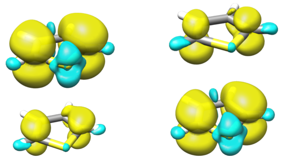
Fig. 15.5 Spin densities for the first two diabatic doublet states of the dithiophene cation.
While the adiabatic spin-densities are evenly distributed over both monomers (50:50), the diabatic spin-densities are each localized mainly on one fragment (87:13).