15. Plotting

pysisyphus offers extensive visualization capabilities via the pysisplot command. All relevant information produced by pysisyphus and the interfaced quantum chemistry programs is dumped to HDF5 files, namely:

Filename	Description
optimization.h5	Produced by all optimizers when dump: True (default).
afir.h5	Contains true and modified energies & forces in AFIR calculations.
forward_irc_data.h5	IRC data from forward run.
backward_irc_data.h5	IRC data from backward run.
finished_irc_data.h5	IRC data from forward & backward run.
overlap_data.h5	From excited state calculations by OverlapCalculator classes.

A help message that shows possible usages of pysisplot is displayed by

pysisplot --help

If needed, results from multiple optimizations are written to different HD5-groups of the same HDF5-file. Available groups can be listed either by the HDF5-tool h5ls or pysisplot --h5_list [hd55 file]. The desired group for visualization is then selected by the --h5_group [group name] argument.

15.1. Example - Diels-Alder reaction

The plotting capabilities of pysisplot are demonstrated for the example of a Diels-Alder reaction between ethene and 1-4-butadiene (see examples/06_diels_alder_xtb_preopt_neb_tsopt_irc) at xtb-GFN2 level of theory. Educts and product of the reaction are preoptimized for 5 cycles, then interpolated in internal coordinates. A chain of states (COS) is optimized loosely via a LBFGS optimizer. The highest energy image (HEI) is employed for a subsequent transition state (TS) optimization. Finally the intrinsic reaction coordinate (IRC) is obtained by means of an Euler-Predictor-Corrector integrator.

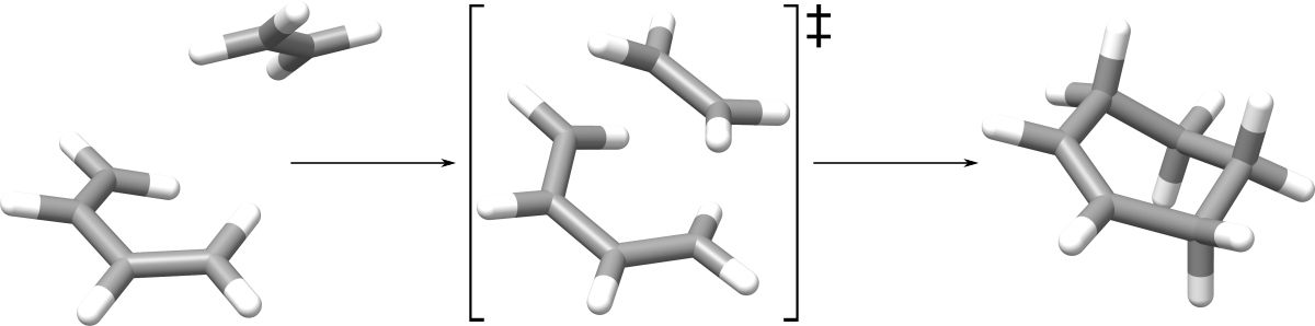
Fig. 15.1 Educts, TS and products of the Diels-Alder reaction between ethene and 1-4-butadiene.

15.1.1. Plotting optimization progress

The progress of an optimization can be plotted via

pysisplot --opt [--h5_fn optimization.h5] [--h5_group opt]

Arguments given in parantheses are the assumed defaults. The result is shown below for the preoptimizations of educts and product.

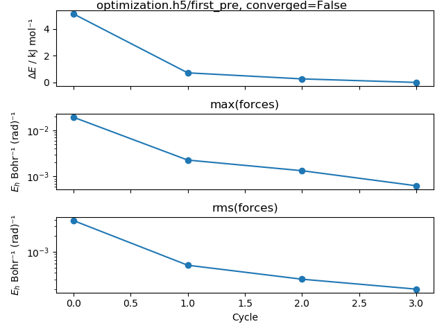
Fig. 15.2 Preoptimization of the Diels-Alader reaction educts ethene + 1,4-butadiene. The upper panel shows the energy change along the optimization. Middle and lower panel show the max and rms of the force. The HDF5 filename and group are noted in the image title.

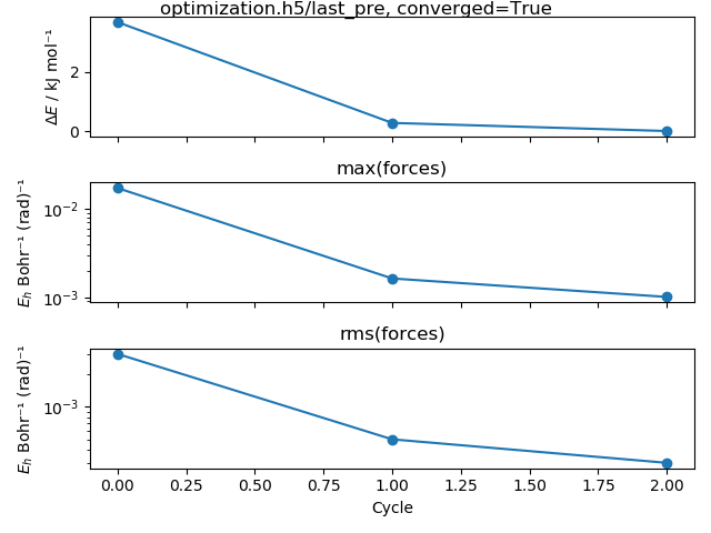
Fig. 15.3 Preoptimization of the Diels-Alader reaction product. Compared to the educts the optimization already converged after 4 cycles.

For COS optimizations all image energies of one optimization cycle are summed into a total energy, which is then plotted in the first panel. pysisplot --opt may not be the best choice in these cases. Use pysisplot --cosens and pysisplot --cosforces instead (see below).

15.1.2. Plotting COS optimization progress

Compared to simple surface-walking optimizations of single molecules, COSs consist of multiple images, each with its own energy and force vector. In this case a simple plot as shown above is not suitable. Instead of pysisplot --opt a better visualization is offered by pysisplot --cosens and pysisplot --cosforces. The latter two commands are compatible with all COS methods available in pysisphus.

pysisplot --cosens [--h5_fn optimization.h5] [--h5_group opt]

This produces three plots.

1. Animated. COS image energies along the optimization.

2. Static. Energies of last optimization cycle.

3. Static. Energies of all cycles with earlier cycles given in a lighter shade and more recent cycles in a darker shade. The last cycle is splined and the position of the splined HEI is indicated.

Please note that equidistant image spacing is assumed for the latter two plots. Here only the two latter plots are shown.

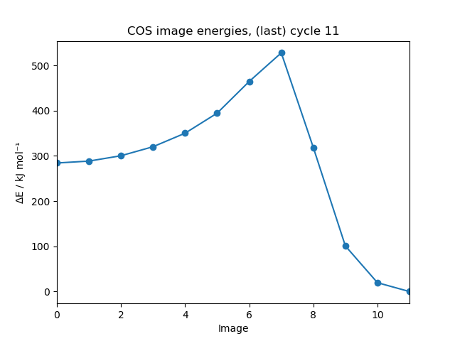
Fig. 15.4 COS image energies of the last (most recent) optimization cycle.

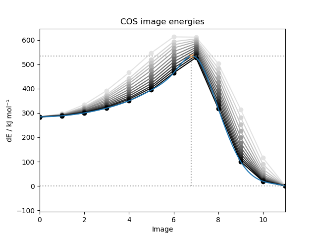
Fig. 15.5 COS image energies of all optimization cycles. Not that the acutal difference between image geometries are not taken into account. Equidistance is assumed. Later (more recent) cycles are given in a darker shade.

The forces acting on the respective COS images can also be plotted.

pysisplot --coforces [--h5_fn optimization.h5] [--h5_group opt]

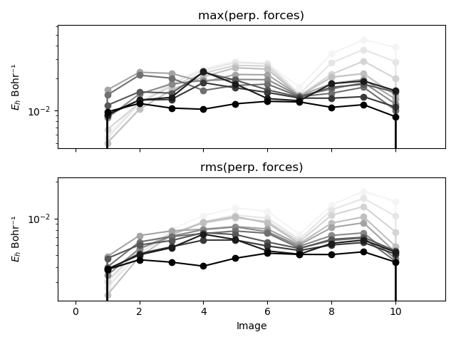
Fig. 15.6 Maximum component and root-mean-square (rms) of the perpendicular component of the force, acting on the COS images.

Please note that nothing is plotted for images 0 and 11, as they remained fixed in the optimization.

15.1.3. Plotting TS-optimization progress

The TS-optimization progress is plotted with pysisplot --opt --h5_group tsopt. Here we explicitly selected a different HDF5 group by --h5_group.

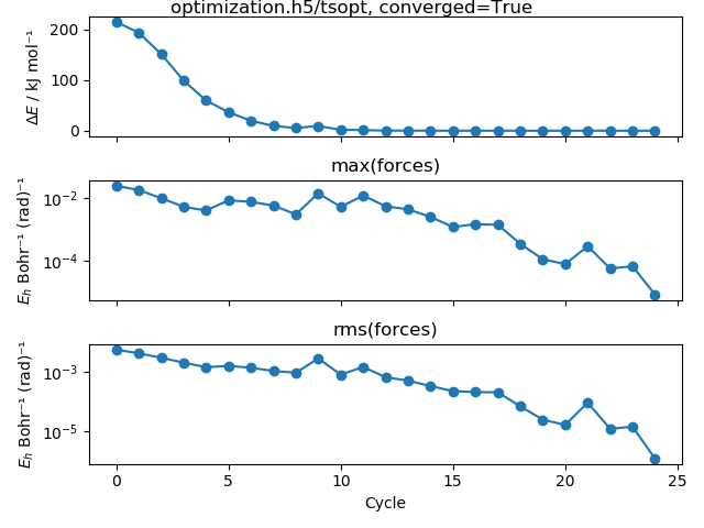
Fig. 15.7 Progress of the TS optimization, started from the HEI.

15.1.4. Plotting the Intrinsic Reaction Coordinate

IRC profiles are easily plotted by

pysisplot --irc

Multiple plots may appear, depending on the progress of the IRC. The IRC coordinate is given in mass-weighted cartesian coordinates, whereas gradients are given in non-mass-weighted units.

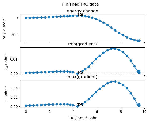
Fig. 15.8 IRC for the Diels-Alder reaction between ethene and 1,4-butadiene.

Evidently the IRC integration failed at the end, as can be seen from the the bunched up points, but unless you want to do some kind of transition-state-theory (TST; not supported by pysisyphus) calculations this should not be a problem.

15.2. Example - AFIR

pysisplot is able to visualize AFIR calculations and to highlight intersting geometries along the optimization. Shown below is an example taken from the AFIR-Paper . By using AFIR the S_N2 between OH^- and fluoromethylene can be forced, yielding methanol and the fluorine anion. The corresponding unit test can be found in the tests/test_afir directory of the repository.

Fig. 15.9 Formation of methanol by means of a S_N2 reaction.

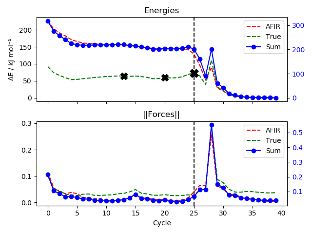
Fig. 15.10 Energy profile and force norms along the S_N2 reaction.

15.3. Example - Excited State Tracking

pysisyphus is aware of excited states (ES) and can track them using various approaches over the course of an optimization or an IRC. By calculating the overlap matrices between ESs at given geometry and a reference geometry pysisyphus can track the desired ES. All relevant data is stored in overlap_data.h5.

Optimizing an ES is demonstrated for the S₁ of the 1H-amino-keto tautomer of Cytosin at the PBE0/def-SVP level of theory. A corresponding test can be found under (tests/test_cytosin_opt). Right after the first optimization cycle a root flip occurs and the S₁ and S₂ switch. The potential energy curves along the optimization are plotted by:

pysisplot --all_energies
pysisplot -a

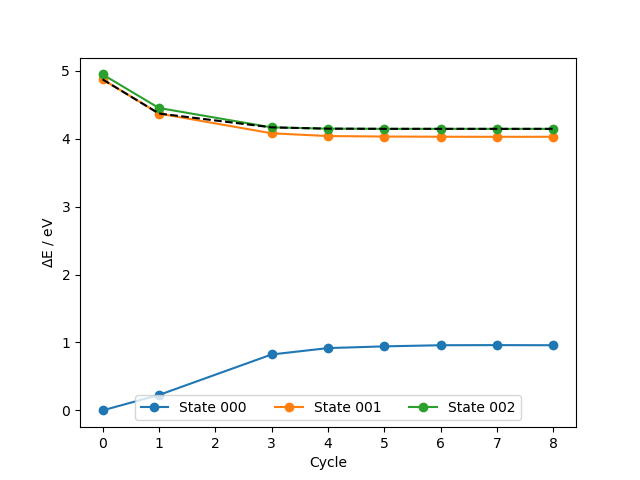
Fig. 15.11 Potential energy curves along the S₁ optimization of the 1H-amino-keto tautomer of Cytosin at the PBE0/def2-SVP level of theory. The root actually followed is indicated by a dashed line.

The calculated overlap matrices can be plotted by:

pysisplot --overlaps
pysisplot -o

If the calculation was set up to calculate charge-density-differences (CDDs) via MultiWFN and to render them via Jmol then the CDD images displayed beside the overlap matrices.

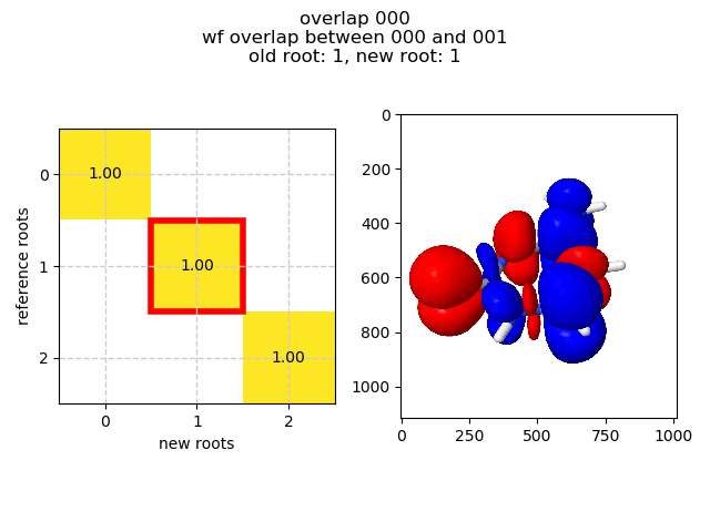
Fig. 15.12 Cytosin S₁ optimization. Overlaps between first and second cycle. No root flips occured. All ES are in the same order as in the reference geometry at cycle 0.

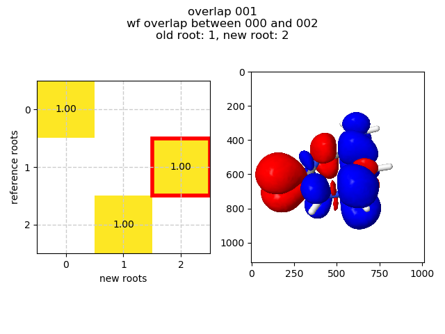
Fig. 15.13 Cytosin S₁ optimization. Overlaps between second and third cycle with root flip. The S₁ and S₂ switch their order.